Visualizing Sorting Algorithms

Introduction

Most developers first learn sorting algorithms by staring at nested loops on a whiteboard. That is usually a mistake.

Sorting is fundamentally a visual process. If you try to memorize the code before you understand how the data actually moves, you will constantly forget how the algorithms work. We need to build an intuition for the mechanics first.

Before we look at the individual visual patterns, we need to talk about the math that makes some algorithms fast and others painfully slow.

Understand the Math (Big O Notation)

When programmers talk about how fast an algorithm is, they do not measure it in seconds. A fast computer will always beat a slow computer in raw seconds. Instead, we measure how the number of steps grows as the amount of data increases.

We write this using Big O notation. It sounds intimidating, but it is just a shorthand for scaling.

Think of the letter $n$ as the number of items you need to sort. If you have ten cards, $n = 10$. If you are sorting a million database rows, $n = 1,000,000$.

Here are the three speeds you will see when analyzing sorting algorithms.

Linear Time: $O(n)$

This means the work scales exactly with the data. If you double the amount of data, the work doubles.

Think of reading a book. If a book has 100 pages, it takes a certain amount of time to read. If it has 200 pages, it takes twice as long. You are doing one unit of work per page. This is incredibly efficient, but it is usually impossible to fully sort an entirely random list in strictly linear time.

Quadratic Time: $O(n^2)$

This is a warning sign for performance. It means for every single item in your list, you have to scan every single other item in your list.

Imagine you are in a room with 10 people, and everyone has to shake hands with everyone else. That is 100 handshakes. If 100 people enter the room, the number of handshakes jumps to 10,000. If you double the data, the work quadruples. An $O(n^2)$ algorithm might run fine on a list of fifty items, but it will completely freeze your application if you run it on fifty thousand items.

Linearithmic Time: $O(n \log n)$

This is the gold standard for sorting. To understand the “log” part, think about looking up a name in a physical phone book.

You do not read every single page (which would be $O(n)$). Instead, you open the book to the middle. If the name you want comes earlier in the alphabet, you rip the book in half, throw away the back half, and look at the middle of the remaining pages. You keep halving the problem.

You can cut a massive dataset in half surprisingly few times before you reach single items. A fast sorting algorithm uses this exact halving trick. If you do $n$ amount of work at each of those halving steps, you get an $O(n \log n)$ speed. It handles massive amounts of data gracefully.

To see the drastic difference between $n^2$ and $n \log n$, we need to watch them run.

Bubble Sort

The math here is straightforward and inefficient. You compare adjacent pairs $n$ times, and you do this for $n$ full passes over the array. Multiplying $n \times n$ gives us the classic $O(n^2)$ worst-case complexity.

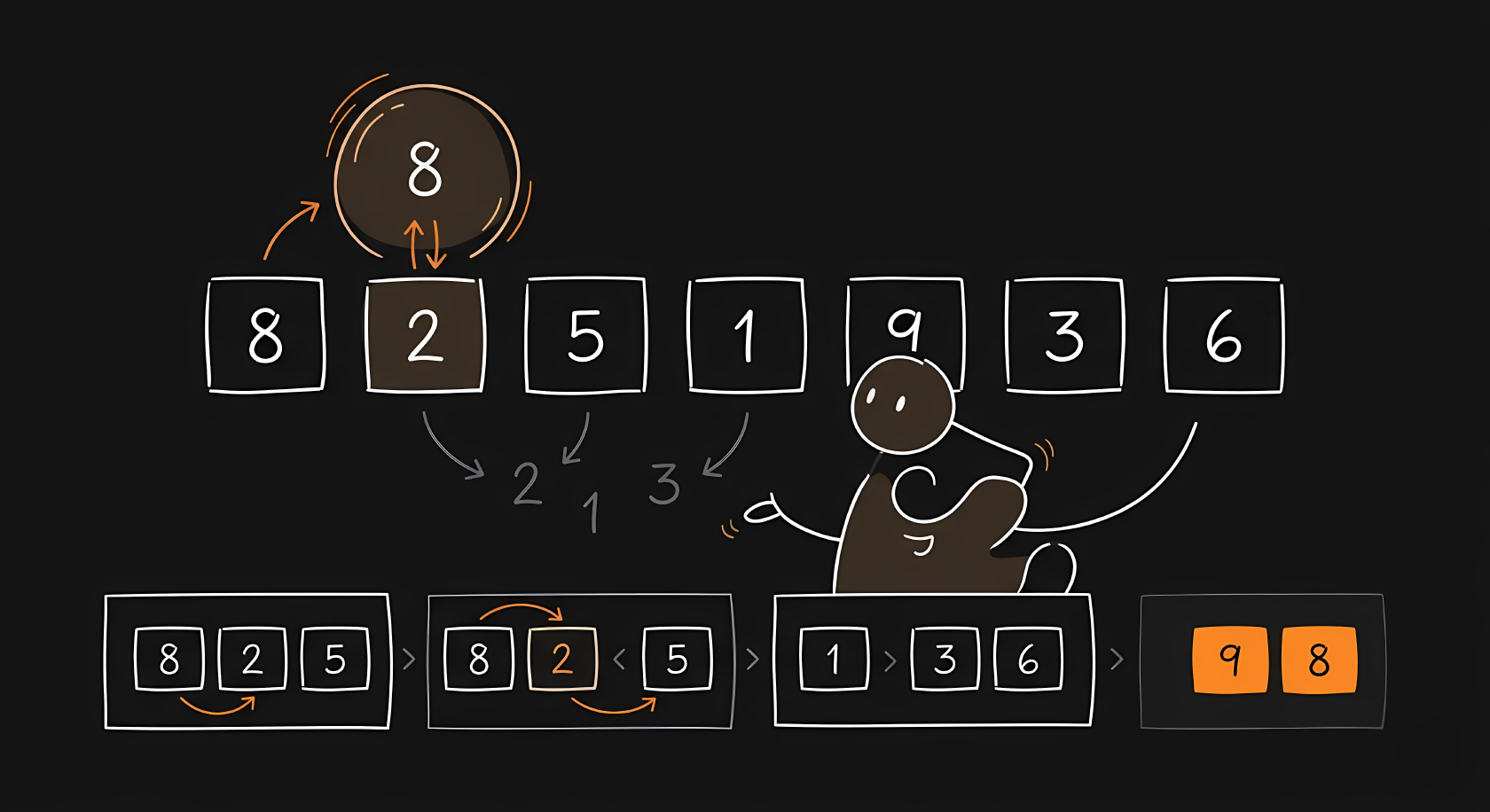
Visually, every element is strictly compared to its immediate neighbor. If the left item is larger, they swap. You will see the largest numbers “bubble” up to the far right side of the screen one by one. It requires multiple full passes over the data until no more swaps are needed.

Here is how that neighbor-swapping logic looks in C. The outer loop controls the passes, and the inner loop pushes the largest remaining item to the right.

void bubbleSort(int arr[], int n) {
    for (int i = 0; i < n - 1; i++) {
        // The last i elements are already in place
        for (int j = 0; j < n - i - 1; j++) {
            if (arr[j] > arr[j + 1]) {
                // Swap the items
                int temp = arr[j];
                arr[j] = arr[j + 1];
                arr[j + 1] = temp;
            }
        }
    }
}

Selection Sort

The math for Selection Sort also resolves to $O(n^2)$. You scan all $n$ items to find the absolute smallest number, taking $n$ steps. Then you scan the remaining $n-1$ items to find the next smallest. Summing $n + (n-1) + (n-2)...$ results in roughly $n^2 / 2$ operations. In Big O notation, we drop the constant half, leaving $n^2$.

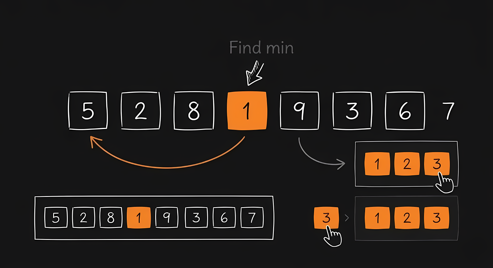
Notice how the visual is split into two strict zones. The left side is perfectly sorted and never touched again. The right side is completely unsorted. The algorithm scans the entire unsorted right side, picks the smallest item, and snaps it onto the end of the sorted left side.

In C, we replicate those two zones. The variable i marks the boundary between the sorted left side and the unsorted right side.

void selectionSort(int arr[], int n) {
    for (int i = 0; i < n - 1; i++) {
        int min_idx = i;

        // Scan the unsorted right side for the smallest item
        for (int j = i + 1; j < n; j++) {
            if (arr[j] < arr[min_idx]) {
                min_idx = j;
            }
        }

        // Swap it to the end of the sorted left side
        int temp = arr[min_idx];
        arr[min_idx] = arr[i];
        arr[i] = temp;
    }
}

Insertion Sort

Insertion sort is mathematically interesting because its speed depends heavily on the initial state of the data. If the list is completely reversed, you must slide each of the $n$ items backward $n$ times, resulting in $O(n^2)$. If the list is already mostly sorted, you only do one quick check per item, giving an incredibly fast $O(n)$.

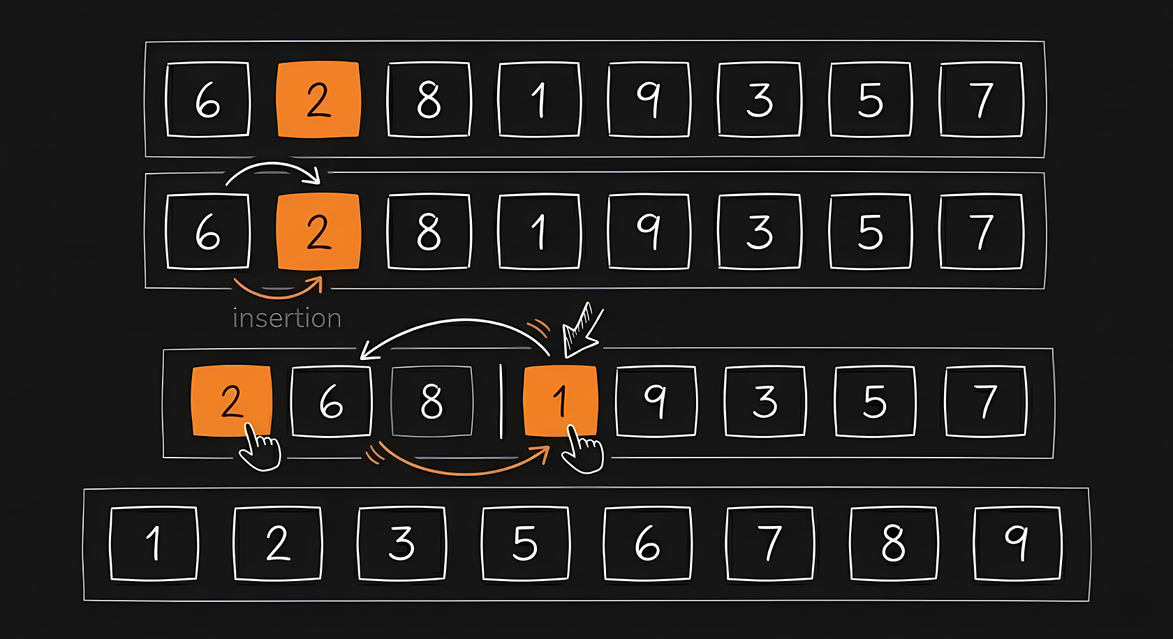
This looks exactly like sorting playing cards in your hand. The algorithm takes one new item from the right side and slides it backward through the left side until it finds its correct resting place.

The C code relies on a while loop that continuously pulls the current item (key) backward as long as the items to its left are larger.

void insertionSort(int arr[], int n) {
    for (int i = 1; i < n; i++) {
        int key = arr[i];
        int j = i - 1;

        // Slide the key backward until it fits
        while (j >= 0 && arr[j] > key) {
            arr[j + 1] = arr[j];
            j = j - 1;
        }

        arr[j + 1] = key;
    }
}

Merge Sort

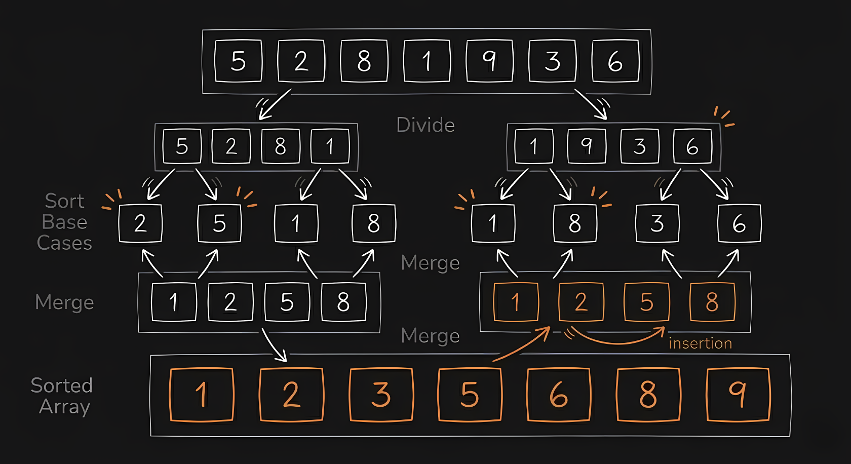
Merge Sort introduces our phone book math. You cut the array in half repeatedly until you are left with single elements. A dataset of $n$ items can be halved $\log n$ times. At each level of cutting, you must merge the items back together in order, which takes $n$ operations. Multiplying the $\log n$ levels by the $n$ merging work gives a consistent $O(n \log n)$ speed.

This is the classic divide and conquer approach. In the video, you will see the data break into tiny fragments immediately. Then, small sorted blocks merge into larger sorted blocks, which merge into even larger blocks until the entire array is unified.

Writing this in C requires two functions. The main function cuts the array in half recursively, and a helper function merges the two sorted halves back together using temporary arrays.

// Helper function to zip two sorted halves together
void merge(int arr[], int left, int mid, int right) {
    int n1 = mid - left + 1;
    int n2 = right - mid;
    int L[n1], R[n2];

    // Copy data into temporary left and right arrays
    for (int i = 0; i < n1; i++)
        L[i] = arr[left + i];

    for (int j = 0; j < n2; j++)
        R[j] = arr[mid + 1 + j];

    int i = 0, j = 0, k = left;

    // Merge them back in order
    while (i < n1 && j < n2) {
        if (L[i] <= R[j]) {
            arr[k++] = L[i++];
        } else {
            arr[k++] = R[j++];
        }
    }

    // Pick up any remaining items
    while (i < n1)
        arr[k++] = L[i++];

    while (j < n2)
        arr[k++] = R[j++];
}

// The main divide function
void mergeSort(int arr[], int left, int right) {
    if (left < right) {
        int mid = left + (right - left) / 2;

        mergeSort(arr, left, mid);      // Cut left half
        mergeSort(arr, mid + 1, right); // Cut right half
        merge(arr, left, mid, right);   // Zip them back together
    }
}

Quick Sort

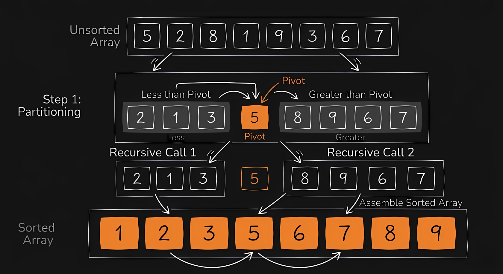
Quicksort relies on probability for its math. You pick a “pivot” element and split the remaining $n$ items into two groups: smaller and larger. If your pivot is close to the median, you effectively cut the problem in half $\log n$ times, giving an excellent $O(n \log n)$ average speed. If you consistently pick the absolute worst pivot, you only reduce the problem size by one each time, devolving to $O(n^2)$.

Visually, it looks highly disorganized. The algorithm picks a pivot, throws everything smaller to the left, and throws everything larger to the right. It then repeats this exact aggressive sorting process for the left and right fragments until everything settles.

In C, we manage this with a partition function that throws items across the pivot line, and a main function that recurses on the left and right sides.

void swap(int* a, int* b) {
    int t = *a;
    *a = *b;
    *b = t;
}

// Throws smaller items left and larger items right
int partition(int arr[], int low, int high) {
    int pivot = arr[high]; // Choosing the last item as the pivot
    int i = (low - 1);

    for (int j = low; j <= high - 1; j++) {
        if (arr[j] < pivot) {
            i++;
            swap(&arr[i], &arr[j]);
        }
    }

    swap(&arr[i + 1], &arr[high]);
    return (i + 1);
}

void quickSort(int arr[], int low, int high) {
    if (low < high) {
        int pi = partition(arr, low, high);

        quickSort(arr, low, pi - 1);  // Sort the left side
        quickSort(arr, pi + 1, high); // Sort the right side
    }
}

Heapsort

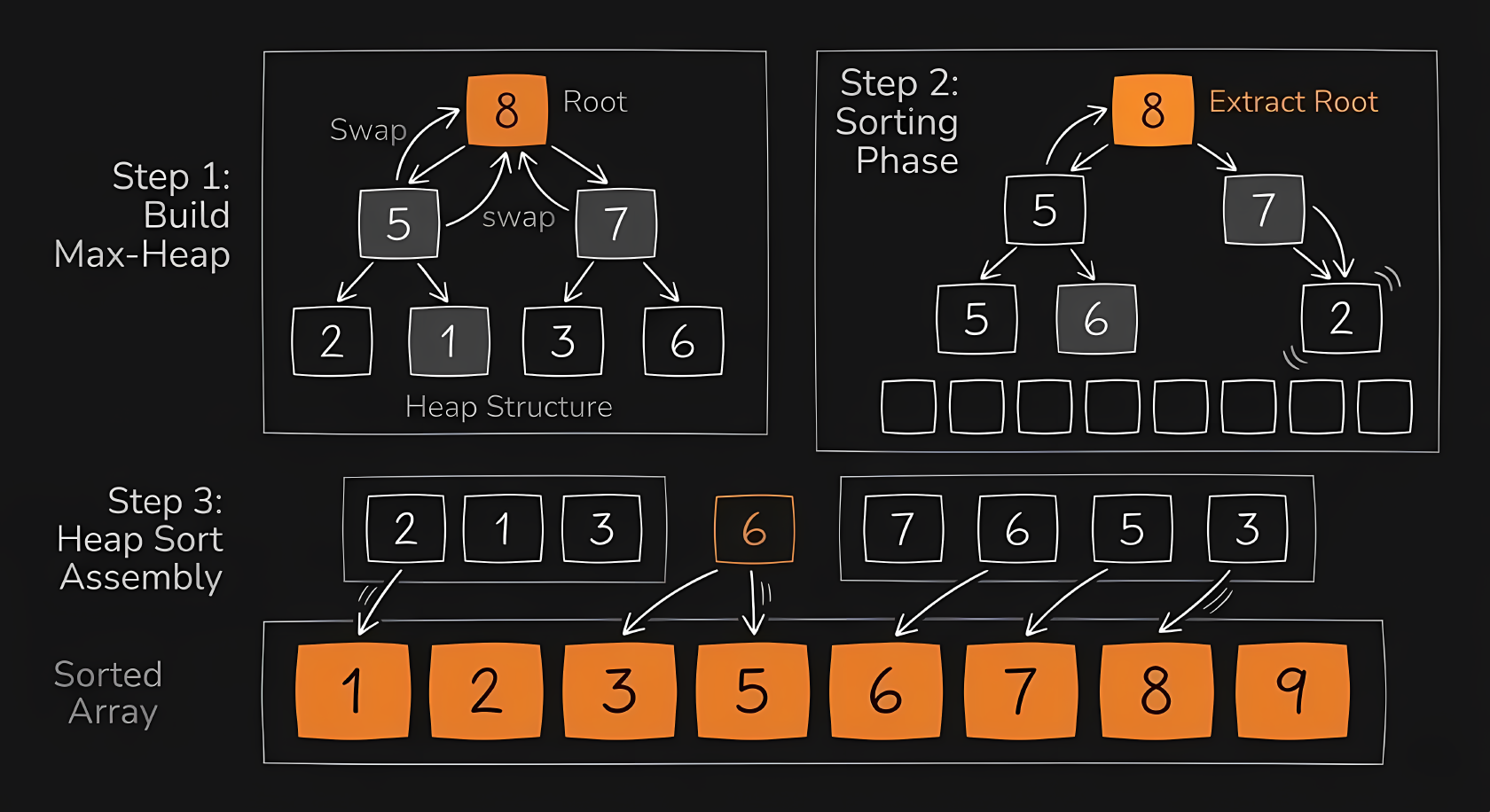
Heapsort guarantees an $O(n \log n)$ time limit by mapping the array into a mathematical binary tree structure. Building the initial tree takes $O(n)$ time. Pulling the largest item off the top of the tree and fixing the branches takes $\log n$ time, and you must do that $n$ times.

The visualization happens in two phases. First, it looks like it is shuffling the data into a very specific, slightly organized mess (the heap). Once the heap is built, you will see the absolute largest item pop off the top and snap to the end of the array, while the rest of the heap quickly repairs itself.

The C implementation requires a heapify function to repair the tree structure. The main sorting function builds the initial tree, then systematically strips the largest item off the top.

void heapify(int arr[], int n, int i) {
    int largest = i;
    int left = 2 * i + 1;
    int right = 2 * i + 2;

    // Find the largest among root, left child, and right child
    if (left < n && arr[left] > arr[largest])
        largest = left;

    if (right < n && arr[right] > arr[largest])
        largest = right;

    // If root is not the largest, swap and repair the affected branch
    if (largest != i) {
        int temp = arr[i];
        arr[i] = arr[largest];
        arr[largest] = temp;

        heapify(arr, n, largest);
    }
}

void heapSort(int arr[], int n) {
    // Phase 1: Build the initial max heap
    for (int i = n / 2 - 1; i >= 0; i--)
        heapify(arr, n, i);

    // Phase 2: Pop the largest item and repair the heap
    for (int i = n - 1; i > 0; i--) {
        int temp = arr[0];
        arr[0] = arr[i];
        arr[i] = temp;

        heapify(arr, i, 0);
    }
}

Shellsort

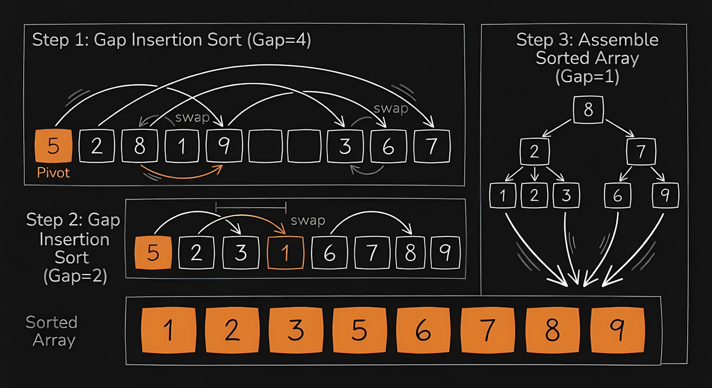
Shellsort is a brilliant mathematical optimization over standard Insertion Sort. Instead of shifting items one position at a time, it shifts them across large gaps, then slowly shrinks the gap down to 1. The exact math depends on the gap sequence you choose, but a good sequence drops the operations down to roughly $O(n^{1.25})$ or $O(n \log^2 n)$.

Notice how elements teleport massive distances early in the process. It is resolving the biggest disorders first. As the video progresses, the comparisons get closer and closer together until the final pass, which is just a simple Insertion Sort cleaning up the remaining minor out of place items.

The C code looks very similar to Insertion Sort, but we wrap the logic in an outer loop that divides the gap size by two on every pass.

void shellSort(int arr[], int n) {
    // Start with a large gap, then reduce the gap
    for (int gap = n / 2; gap > 0; gap /= 2) {

        // Do a gapped insertion sort for this gap size
        for (int i = gap; i < n; i += 1) {
            int temp = arr[i];
            int j;

            // Shift earlier gap-sorted elements up until the correct location is found
            for (j = i; j >= gap && arr[j - gap] > temp; j -= gap) {
                arr[j] = arr[j - gap];
            }

            arr[j] = temp;
        }
    }
}

Comb Sort

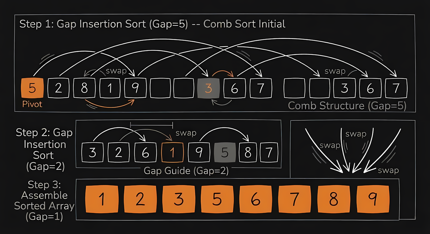
Comb Sort is Bubble Sort with math applied to fix its worst flaw. Bubble Sort struggles with “turtles” (small numbers stuck at the far right end of the array that take forever to bubble backward). Comb Sort compares items separated by a large gap and shrinks the gap by a specific mathematical ratio (usually 1.3) each pass. This clears the turtles out early, pushing the average performance near $O(n \log n)$.

The intuition is exactly like running a wide tooth comb through tangled hair before switching to a fine tooth comb. The early, wide gap comparisons aggressively push the small values to the left side of the screen, completely preventing the slow crawling behavior seen in standard Bubble Sort.

The C code sets the initial gap to the size of the array and repeatedly divides it by 1.3. Once the gap hits 1, it acts exactly like Bubble Sort to finish the job.

void combSort(int arr[], int n) {
    int gap = n;
    int swapped = 1;

    // Run until the gap is 1 and no swaps occur
    while (gap != 1 || swapped == 1) {
        // Shrink the gap by the 1.3 factor
        gap = (gap * 10) / 13;
        if (gap < 1) {
            gap = 1;
        }

        swapped = 0;

        // Compare items across the current gap
        for (int i = 0; i < n - gap; i++) {
            if (arr[i] > arr[i + gap]) {
                int temp = arr[i];
                arr[i] = arr[i + gap];
                arr[i + gap] = temp;
                swapped = 1;
            }
        }
    }
}

Real World Usage

In daily engineering work, you will almost never write your own sorting algorithm from scratch in C or any other language.

Modern programming languages already handle this for us. When you call a built in sorting function, the compiler or interpreter relies on highly optimized routines. They often use hybrid approaches, like Timsort (which combines Merge Sort and Insertion Sort) or Introsort (which begins with Quicksort and switches to Heapsort if things go wrong), to handle real world data efficiently.

So why bother learning how they work?

Understanding these patterns changes how you think about data. When you know why an $O(n^2)$ operation grinds to a halt on a large dataset, you make better architectural decisions. You learn to recognize when a problem can be solved faster by splitting it in half. You stop guessing why your application is slow and start measuring how your data is actually moving.